Simple Linear Regression in R

Regression shows a line or curve that passes through all the data points on the target-predictor graph in such a way that the vertical distance between the data points and the regression line is minimum

What is Linear Regression?

Linear Regression is a commonly used type of predictive analysis. Linear Regression is a statistical approach for modelling the relationship between a dependent variable and a given set of independent variables. It is predicted that a straight line can be used to approximate the relationship. The goal of linear regression is to identify the line that minimizes the discrepancies between the observed data points and the line’s anticipated values.

There are two types of linear regression.

Simple Linear Regression
Multiple Linear Regression

Let’s discuss Simple Linear regression using R Programming Language .

Simple Linear Regression in R

In Machine Learning Linear regression is one of the easiest and most popular Machine Learning algorithms.

It is a statistical method that is used for predictive analysis.
Linear regression makes predictions for continuous/real or numeric variables such as sales, salary, age, product price, etc.
Linear regression algorithm shows a linear relationship between a dependent (y) and one or more independent (y) variables, hence called as linear regression. Since linear regression shows the linear relationship, which means it finds how the value of the dependent variable changes according to the value of the independent variable.

Linear Regression Line

A linear line showing the relationship between the dependent and independent variables is called a regression line. A regression line can show two types of relationship:

Positive Linear Relationship: If the dependent variable increases on the Y-axis and the independent variable increases on the X-axis, then such a relationship is termed as a Positive linear relationship.
Negative Linear Relationship: If the dependent variable decreases on the Y-axis and independent variable increases on the X-axis, then such a relationship is called a negative linear relationship.

Assumptions of Linear Regression

Below are some important assumptions of Linear Regression. These are some formal checks while building a Linear Regression model, which ensures to get the best possible result from the given dataset.

Linear relationship between the features and target: Linear regression assumes the linear relationship between the dependent and independent variables.
Small or no multicollinearity between the features: Multicollinearity means high-correlation between the independent variables. Due to multicollinearity, it may difficult to find the true relationship between the predictors and target variables. Or we can say, it is difficult to determine which predictor variable is affecting the target variable and which is not. So, the model assumes either little or no multicollinearity between the features or independent variables.
Homoscedasticity: Homoscedasticity is a situation when the error term is the same for all the values of independent variables. With homoscedasticity, there should be no clear pattern distribution of data in the scatter plot. We want to have homoscedasticity. To check for homoscedasticity we use a scatterplot of the residuals against the independent variable. Once this plot is created we are looking for a rectangular shape. This rectangle is indicative of homoscedasticity. If we see a cone shape, that is indicative of heteroscedasticity.
Normal distribution of error terms: Linear regression assumes that the error term should follow the normal distribution pattern. If error terms are not normally distributed, then confidence intervals will become either too wide or too narrow, which may cause difficulties in finding coefficients. It can be checked using the q-q plot. If the plot shows a straight line without any deviation, which means the error is normally distributed.
No autocorrelations: The linear regression model assumes no autocorrelation in error terms. If there will be any correlation in the error term, then it will drastically reduce the accuracy of the model. Autocorrelation usually occurs if there is a dependency between residual errors.

It is a statistical method that allows us to summarize and study relationships between two continuous (quantitative) variables. One variable denoted x is regarded as an independent variable and the other one denoted y is regarded as a dependent variable. It is assumed that the two variables are linearly related. Hence, we try to find a linear function that predicts the response value(y) as accurately as possible as a function of the feature or independent variable(x).

Y = β₀ + β₁X + ε

The dependent variable, also known as the response or outcome variable, is represented by the letter Y.
The independent variable, often known as the predictor or explanatory variable, is denoted by the letter X.
The intercept, or value of Y when X is zero, is represented by the β₀.
The slope or change in Y resulting from a one-unit change in X is represented by the β₁.
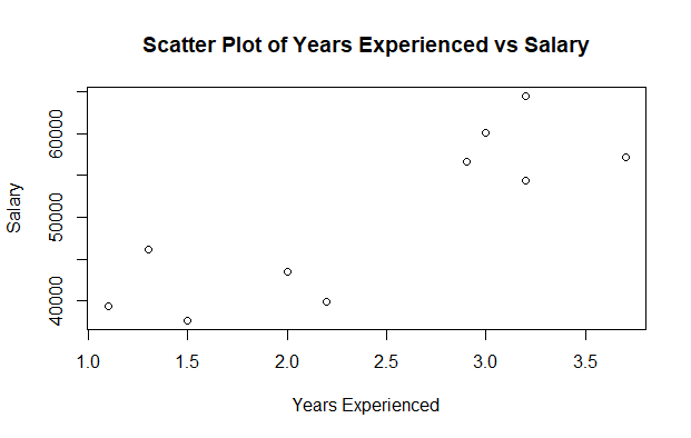
The error term or the unexplained variation in Y is represented by the ε.

For understanding the concept let’s consider a salary dataset where it is given the value of the dependent variable(salary) for every independent variable(years experienced).

Salary dataset:

For general purposes, we define:

x as a feature vector, i.e x = [x_1, x_2, …., x_n],
y as a response vector, i.e y = [y_1, y_2, …., y_n]
for n observations (in the above example, n=10).

First we convert these data values into R Data Frame

R

# Create the data frame data <- data.frame ( Years_Exp = c (1.1, 1.3, 1.5, 2.0, 2.2, 2.9, 3.0, 3.2, 3.2, 3.7), Salary = c (39343.00, 46205.00, 37731.00, 43525.00, 39891.00, 56642.00, 60150.00, 54445.00, 64445.00, 57189.00)

Scatter plot of the given dataset

R

# Create the scatter plot plot (data$Years_Exp, data$Salary, xlab = "Years Experienced" , ylab = "Salary" , main = "Scatter Plot of Years Experienced vs Salary" )

Output:

Linear Regression in R

Now, we have to find a line that fits the above scatter plot through which we can predict any value of y or response for any value of x
The line which best fits is called the Regression line.

The equation of the regression line is given by:

y = a + bx

Where y is the predicted response value, a is the y-intercept, x is the feature value and b is the slope.
To create the model, let’s evaluate the values of regression coefficients a and b. And as soon as the estimation of these coefficients is done, the response model can be predicted. Here we are going to use the Least Square Technique .

The principle of least squares is one of the popular methods for finding a curve fitting a given data. Say $(x_1, y_1), (x_2, y_2),\cdots,(x_n, y_n)$ be n observations from an experiment. We are interested in finding a curve

Closely fitting the given data of size ‘n’. Now at x=x1 while the observed value of y is y1 the expected value of y from curve (1) is f(x1). Then the residual can be defined by…

Similarly, residuals for x2, x3…xn are given by …
$e_2=y_2-f(x_2) \\ \vdots \\ e_n=y_n-f(x_n)$
While evaluating the residual we will find that some residuals are positives and some are negatives. We are looking forward to finding the curve fitting the given data such that residual at any xi is minimum. Since some of the residuals are positive and others are negative and as we would like to give equal importance to all the residuals it is desirable to consider the sum of the squares of these residuals. Thus we consider:

and find the best representative curve.

Least Square Fit of a Straight Line

Suppose, given a dataset of n observation from an experiment. And we are interested in fitting a straight line.

to the given data.
Now consider:

Now consider the sum of the squares of ei
$\begin{aligned} E&=\sum_{i=1}^{n} e_{i}^{2} \\ &=\sum_{i=1}^{n}\left[y_{i}-\left(a x_{i}+b\right)\right]^{2} \end{aligned}$

Note: E is a function of parameters a and b and we need to find a and b such that E is minimum and the necessary condition for E to be minimum is as follows:

This condition yields:
$\begin{aligned} \frac{\partial E}{\partial a}& =0 \\ \sum_{i=1}^{n} 2 x_{i}\left[y_{i}-\left(a x_{i}+b\right)\right]&=0 \\ \sum_{i=1}^{n} \left[y_{i}-\left(a x_{i}+b\right)\right]&=0 \\ a \sum_{i=1}^{n} x_{i}+n b & =\sum_{i=1}^{n} y_{i} \end{aligned}$
The above two equations are called normal equations which are solved to get the value of a and b.
The Expression for E can be rewritten as:
$E=\sum_{i=1}^{n} y_{i}^{2}-a \sum_{i=1}^{n} x_{i} y_{i}-b \sum_{i=1}^{n} y_{i}$
The basic syntax for regression analysis in R is

lm(Y ~ model)

where Y is the object containing the dependent variable to be predicted and the model is the formula for the chosen mathematical model.
The command lm( ) provides the model’s coefficients but no further statistical information.

The following R code is used to implement Simple Linear Regression: